How to design the Simplest OrthoK lens with Wolfram Language(5)

For the convenience of subsequent analysis, let's first reorganize the code. There are some simple tricks in Wolfram language, such as using Module to mark local variables. It's not difficult to write, we just need to give the code we've already written to GPT4 and let AI help to tidy up and simplify it.

• First is the function to calculate the parameters of orthokeratology lenses:

orthoKParameters[Reye_,Qeye_,Rx_,JF_,BCD_,RCwidth_,ACwidth_,PCD_,PCtear_] := Module[{RCD, ACD, z, BCRfunc, BCR, ACresult, PCresult, RCresult},
  RCD=BCD+2*RCwidth;
  ACD=RCD+2*ACwidth;

  z[R_,Q_,D_, z0_]:=(
    c=1/R;
    r=D/2;
    (c* r^2)/ (1+Sqrt[1-(1+Q)*c^2* r^2]) + z0);

  BCRfunc[Reyeinside_,Rxinside_,JFinside_]:=337.5/(337.5/Reyeinside+Rxinside-JFinside);

  BCR = BCRfunc[Reye,Rx,JF];
 BCz0=-0.003;
 
 RCresult=Solve[
    {z[ BCR, 0, BCD, BCz0] == z[RCR,0,BCD,RCz0],
    z[ Reye, Qeye, RCD, 0] ==z[RCR,0,RCD,RCz0]},
    {RCR,RCz0}];
RCR=RCresult[[1]][[1,2]];
RCz0=RCresult[[1]][[2,2]];

  ACresult=NSolve[{
    z[ACR,0,RCD,ACz0]==z[Reye, Qeye,RCD,0],
    z[ACR,0, ACD, ACz0]==z[Reye, Qeye, ACD, 0]},
    {ACR,ACz0}];
ACR=ACresult[[1]][[1,2]];
ACz0=ACresult[[1]][[2,2]];
 

 PCresult=NSolve[{
    z[Reye, Qeye, ACD, 0]==z[PCR,0,ACD,PCz0],
    z[Reye, Qeye, PCD, 0]==z[PCR,0,PCD,PCz0]+PCtear },
    {PCR,PCz0}];
PCR=PCresult[[1]][[1,2]];
PCz0=PCresult[[1]][[2,2]];

  
  {BCR,RCR,ACR,PCR,BCD,RCD,ACD,PCD,BCz0,RCz0,ACz0,PCz0}
]

• Then, based on these parameters, we can describe the sag height of the posterior surface of the orthokeratology lens with a piecewise function:

orthoKlens[param_,x_]:= Module[{z},
z[R_,Q_,D_, z0_]:=(
    c=1/R;
    r=D/2;
    (c* r^2)/ (1+Sqrt[1-(1+Q)*c^2* r^2]) + z0);
Piecewise[
{
{z[param[[1]], 0, 2 * x, param[[9]]], 0 <= x < param[[5]] / 2},
{z[param[[2]],0,2*x,param[[10]]], param[[5]] / 2 <= x <param[[6]] / 2},
{z[param[[3]], 0, 2 * x, param[[11]]], param[[6]]/ 2 <= x < param[[7]] / 2},
{z[param[[4]], 0, 2 * x, param[[12]]], param[[7]] / 2 <= x < param[[8]] / 2}
}
]
]

• Similarly, we can also define a function to describe the sag height of the corneal surface of the eye. It's actually just a simple conic function:

Eye[R_,Q_,r_]:=Module[{c},
     c=1/R;
    (c* r^2)/ (1+Sqrt[1-(1+Q)*c^2* r^2])]

• By calculating the difference in sag height between the two, we can calculate the thickness of the tear film. The tear film will not be negative, so if the minimum thickness of the tear film is negative, it should be moved to 0. Considering our design, the minimum value will only appear at the starting point of the BC arc, the starting point of the AC arc, and the end point of the AC arc:

SagDiff[Rp_,Qp_, param_, x_]:=Eye[Rp,Qp,x]-orthoKlens[param,x]
Tear[Rp_,Qp_, param_, x_]:=SagDiff[Rp,Qp, param, x]-Min[
{SagDiff[Rp,Qp, param, 0],SagDiff[Rp,Qp, param, param[[6]]/2],SagDiff[Rp,Qp, param, param[[7]]/2]}]

• Finally, for the convenience of analysis, we also need to make a plotting function that can draw the thickness of the tear film and simulate the situation of fluorescein staining in green:

DrawTear[Rp_,Qp_,params]:=Module[{PCD, plot1, plot2},
PCD=params[[8]];
plot1 = Plot[Tear[Rp,Qp,params,Abs[x]],{x,-PCD/2,PCD/2}];
plot2 = DensityPlot[20*(If[Sqrt[x^2 + y^2] <= PCD/2, Tear[Rp,Qp,params,Sqrt[x^2 + y^2]], None]), 
{x, -PCD/2, PCD/2}, {y, -PCD/2, PCD/2}, 
ColorFunction -> (Blend[{Black, Green}, #] &), ColorFunctionScaling -> False,PlotPoints -> 100];
GraphicsColumn[{plot1, plot2}]
]

With the above preparations done, we can start the analysis.

We first generate the parameters of an orthokeratology lens, corresponding to the corneal anterior surface radius of curvature = 7.5, Q = -0.2, Rx = -3, etc.:

params=orthoKParameters[7.5,-0.2,-3,0.75,5.5,1,1,11,0.1];

• We assume that a patient comes in, his/her corneal anterior surface radius of curvature is also exactly 7.5, and the Q value is -0.2, so it is a perfect fit at this time. By the way, I modified the distance setting between the BC starting point and the cornea, it should not be in complete contact, there will be a few microns of gap, I left 3 microns:

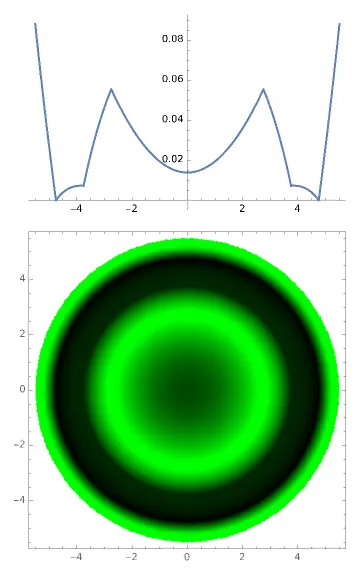
DrawTear[7.5, -0.2, params]

At this time, the starting and ending points of the AC arc are in contact with the cornea, so the thickness of the tear film at these two positions = 0. The fluorescein map shows a clear black ring indicating the range of the AC arc.

• The second patient comes in, his/her corneal anterior surface radius of curvature is also exactly 7.5, but the Q value is not -0.2, but -0.25:

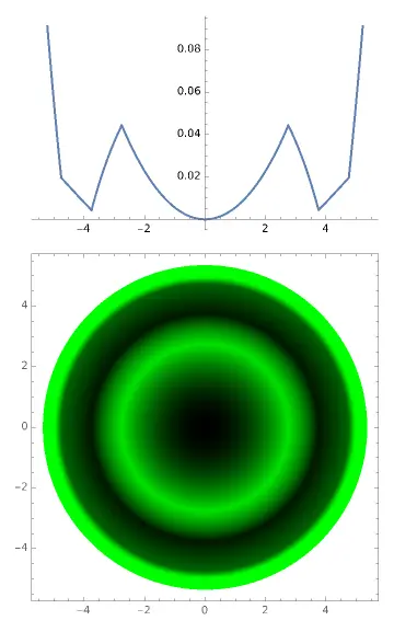
DrawTear[7.5, -0.25, params]

At this time, because the patient's Q value is different from the model eye we used in the design, it can't match perfectly, and the starting point of the AC arc is raised. The fluorescein map shows that the inner edge of the AC ring is a bit blurry. Yes, when you are seeing patients clinically, if you feel that the stained edge corresponding to the AC arc is a bit blurry, it means that it is not in contact with the cornea. At the same time, the distance between the corneal center and the BC arc has increased. According to the current orthokeratology theory, the shaping force is determined by the thickness difference of the tear film at different positions. The maximum force is related to the ratio of the maximum and minimum tear film thickness. Now this ratio has decreased, the shaping force will weaken. At the same time, because the RC arc has also been raised, when the shaping force is insufficient, it may be difficult to shape the cornea into a local "convex lens" in the RC arc area, so the peripheral myopia defocus formed may be insufficient, resulting in insufficient ability to control the progression of myopia. This child may have a faster rate of myopia progression.

• The third patient comes in, his/her corneal anterior surface radius of curvature is also exactly 7.5, but the Q value is not -0.2, but -0.10

DrawTear[7.5, -0.10, params]

This situation is very bad, the patient's corneal center directly contacts the center of the orthokeratology lens, and the AC arc cannot touch the cornea at all, and cannot play a supporting role. At this time, the lens will tilt like a seesaw until one side of the AC arc starting point touches the cornea, at least forming two points of support, before it will stop. If you let this patient go during the fitting, then the next time you review, when you do the corneal topography, you will find that the lens is displaced. If the displacement is severe, you have to let the patient stop wearing it, and then change the lens.

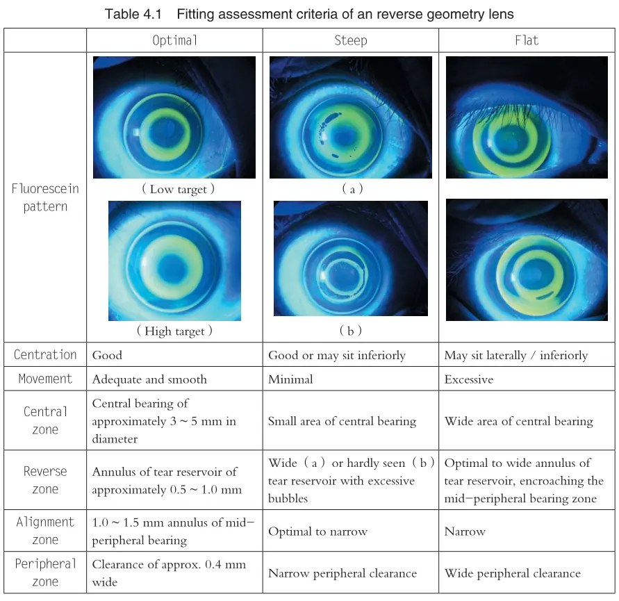
Now please read Chapter 4 of "Orthokeratology Practice", Table 4.1, to see if it can deepen your understanding of orthokeratology lens fitting.