For the sake of analysis, we first consolidate our previous calculations into a piecewise function:
OrthoK[x_] = Piecewise[
    {
      {z[BCR, 0, 2 * x, 0], 0 <= x < BCD / 2},
      {RCresult[[1, 2]]* x + RCresult[[2, 2]], BCD / 2 <= x < RCD / 2},
      {z[ACresult[[1, 2]], 0, 2 * x, ACresult[[2, 2]]], RCD / 2 <= x < ACD / 2},
      {z[PCresult[[1, 2]], 0, 2 * x, PCresult[[2, 2]]], ACD / 2 <= x < PCD / 2}
    }
  ]
Similarly, we can also write a function for the sagittal height of the corneal surface:
Eye[Reye_, Qeye_, x_] = z[Reye, Qeye, 2 * x, 0]
Therefore, the difference in sagittal height between the corneal surface and the posterior surface of the orthokeratology lenses represents the thickness of the tear film layer. We can plot this as follows:
Plot[Eye[Reye, Qeye, x] - OrthoK[x], {x, PCD/2}]
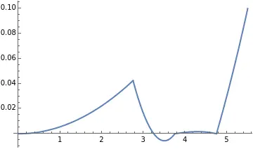
Well, this is a bit awkward. The RC arc cannot be directly connected by a straight line from the end of the BC arc to the beginning of the AC arc, as part of it will be blocked by the cornea.
In this case, we can actually practice a slightly more advanced technique - we can infer the required shape of the RC arc from the thickness of the tear film. For example, I want the tear film thickness at the RC arc position to remain constant.
Since the tear film thickness = Eye[Reye, Qeye, x] - OrthoK[x]
If we want it to be constant, without any jumps, then it should be equal to the tear film thickness at the end of the BC arc, which is
OrthoK[x] = z[Reye, Qeye, 2 * x, 0] + z[BCR, 0, BCD, 0] - z[Reye, Qeye, BCD, 0]
The resulting tear film thickness is as follows:
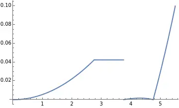
Looking at it this way, one end is connected, but there is still a jump at the other end, which may cause discomfort. So, we force it, allowing the tear film thickness to gradually decrease to zero. We insert a part that decreases linearly,
-(z[BCR,0,BCD,0]-z[Reye,Qeye,BCD,0])/(RCD/2-BCD/2)*(x-BCD/2)
So, the piecewise function for the posterior surface of the orthokeratology lens looks like this:
OrthoK[x_]=Piecewise[
    {
      {z[BCR, 0, 2 * x, 0], 0 <= x < BCD / 2},
      {z[Reye,Qeye,2*x,0]+z[BCR,0,BCD,0]-z[Reye,Qeye,BCD,0]-(z[BCR,0,BCD,0]-z[Reye,Qeye,BCD,0])/(RCD/2-BCD/2)*(x-BCD/2),
			BCD / 2 <= x < RCD / 2},
      {z[ACresult[[1, 2]], 0, 2 * x, ACresult[[2, 2]]], RCD / 2 <= x < ACD / 2},
      {z[PCresult[[1, 2]], 0, 2 * x, PCresult[[2, 2]]], ACD / 2 <= x < PCD / 2}
    }
  ]
The tear film thickness looks like this:
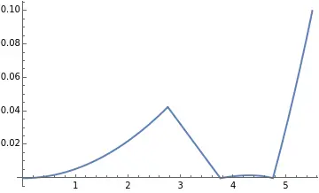
Remember, this is the tear film thickness profile of a perfectly fitted orthokeratology lens.
We can use DensityPlot to draw the image of the tear film thickness rotating around the axis, using color to represent depth, where black = 0, and the deeper the green, the thicker the tear film. Thus, we can get a simulated fluorescein staining image.
DensityPlot[20*(If[Sqrt[x^2 + y^2] <= PCD/2, Eye[Reye, Qeye, Sqrt[x^2 + y^2]] - OrthoK[Sqrt[x^2 + y^2]], None]),
{x, -PCD/2, PCD/2}, {y, -PCD/2, PCD/2},
ColorFunction -> (Blend[{Black, Green}, #] &), ColorFunctionScaling -> False,PlotPoints -> 100]

As can be seen, the central area is black, then gradually turns green, reaching the brightest green ring at the junction of BC and RC. This is the deepest part of the tear film, then it quickly fades. In the AC arc area, if the "fit" is good, it should be very close to the cornea, so the color of the fluorescein is close to black. After leaving the AC arc and entering the PC arc, in order to generate tear exchange, there is some elevation, and the color of the fluorescein quickly deepens until the edge.
In the next section, we can see what happens when the curvature radius and Q value of the orthokeratology lens do not match with the cornea?